Spin-plotting routine (2D)

Here you will find a pre-defined function that can plot the set of spin directions from vampire's output file as a 2D plot.

Definition of the plotting function

Execute the cell below to have the function defined

import numpy as np
from tqdm import tqdm
import matplotlib
from mpl_toolkits.axes_grid1 import make_axes_locatable
import matplotlib.pyplot as plt


def plot_spins(
    filename,
    scale=1.0,
    color_mode="z",
    color_projection=None,
    colormap="bwr",
    vmin=None,
    vmax=None,
    xrange=None,
    yrange=None,
    zrange=None,
):
    # Load data
    data = np.loadtxt(filename, skiprows=1)

    # Make a cut if needded
    if xrange is not None:
        data = data[xrange[0] <= data[:, 0]]
        data = data[data[:, 0] <= xrange[1]]
    if yrange is not None:
        data = data[yrange[0] <= data[:, 1]]
        data = data[data[:, 1] <= yrange[1]]
    if zrange is not None:
        data = data[zrange[0] <= data[:, 2]]
        data = data[data[:, 2] <= zrange[1]]

    print(f"Plotting {data.shape[0]} spins after the real-space cut")

    # Compute color values
    if color_mode == "z":
        color_projection = [0.0, 0.0, 1.0]
    elif color_mode == "y":
        color_projection = [0.0, 1.0, 0.0]
    elif color_mode == "x":
        color_projection = [1.0, 0.0, 0.0]
    elif color_mode == "projection":
        if color_projection is None:
            raise ValueError(
                f"Expected vector for color_projection, got '{color_projection}'"
            )
    else:
        raise ValueError(
            f"Expected 'z', 'y', 'x' or 'projection' for color_mode, got '{color_mode}'"
        )
    color_projection = color_projection / np.linalg.norm(color_projection)
    colors_values = data[:, 3:] @ color_projection

    # Get the normalizer for color values
    if vmin is None:
        vmin = colors_values.min()
    if vmax is None:
        vmax = colors_values.max()

    # Plot all vectors
    fig, ax = plt.subplots()

    im = ax.scatter(
        x=data[:, 0],
        y=data[:, 1],
        s=2 * scale,
        c=colors_values,
        cmap=colormap,
        vmin=vmin,
        vmax=vmax,
    )

    divider = make_axes_locatable(ax)
    cax = divider.append_axes("right", size="5%", pad=0.05)

    fig.colorbar(im, cax=cax)

    print("All spins are processed, starting to show the plot ...")

    # Show the plot
    fig.show()

Explanation for the parameters

You have to provide one parameter

• filename : str

  Name of the file with spin positions and directions.

Other parameters are optional. They control the appearance of the plot:

• scale : float, default 1.0

  This parameter controls the scale of the spin vectors length, play with this value for better-looking result. Increase to make spin vectors appear longer.

• color_mode : str, default "z"

  What value to use for coloring of the spins. Supported:

  • "z" - use z components

  • "y" - use y components

  • "x" - use x components

  • "projection" - use projection along color_projection.

• color_projection : (3,) array-like

  Direction for the spin projection to use for coloring. Used if color_mode = "projection".

• colormap : str, default "bwr"

  Any colormap supported by matplotlib. See https://matplotlib.org/stable/users/explain/colors/colormaps.html for supported names.

• vmin : float, optional

  min value for color value normalization.

• vmax : float, optional

  max value for color value normalization.

• xrange : tuple of 2 float

  Specifies the real-space range on the graph that is plotted. Use it to cut the regions that you want to plot.

• yrange : tuple of 2 float

  Specifies the real-space range on the graph that is plotted. Use it to cut the regions that you want to plot.

• zrange : tuple of 2 float

  Specifies the real-space range on the graph that is plotted. Use it to cut the regions that you want to plot.

Plot with all values set to defaults.

plot_spins("spins-00000020.txt")

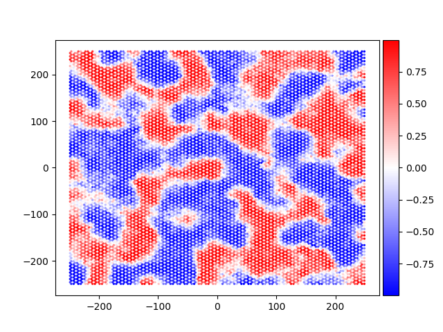
Plotting 12108 spins after the real-space cut
All spins are processed, starting to show the plot ...

Plot a real-space cut.

plot_spins("spins-00000020.txt", xrange=(-20, 20), yrange=(-20, 20), scale=10)

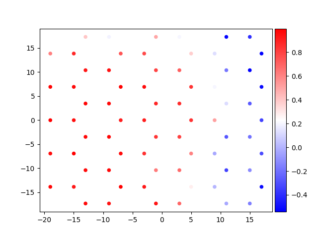
Plotting 71 spins after the real-space cut
All spins are processed, starting to show the plot ...

Plot with coloring according to the value of s_y

plot_spins(
    "spins-00000020.txt",
    xrange=(-20, 20),
    yrange=(-20, 20),
    scale=10,
    color_mode="y",
)

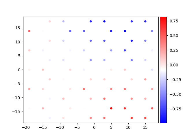
Plotting 71 spins after the real-space cut
All spins are processed, starting to show the plot ...