(extra) K-points with wulfric

Tutorial tasks

• Get kpoints for future dispersion calculations with wulfric.

• (extra) Visualize Brillouin zone, k-points and k-path with wulfric.PlotlyEngine.

• (extra) Create a crystal on FCC lattice with wulfric. Visualize and compare primitive and conventional cells. Compute k-points, k-path. Compare reciprocal cell of conventional cell, reciprocal cell of primitive cell and wulfric.Kpoints.rcell.

One way to get a set of k-points and a k-path in reciprocal space is to use wulfric package.

We recommend to use its wulfric.Kpoints interface. Here we provide not the most straightforward way to interact with it, but the one that gives access to symmetry information. Note that symmetry search in wulfric is powered by spglib.

Wulfric operates on the crystal structure. First, get the information from spglib via wulfric's interface to it.

import wulfric
import magnopy

spinham = magnopy.examples.cubic_ferro_nn(S=1)

spglib_data = wulfric.get_spglib_data(
    cell=spinham.cell,
    atoms=spinham.atoms,
)

Next, display the information about the space group or Bravais lattice type

print(spglib_data.space_group_number)
print(spglib_data.crystal_family + spglib_data.centring_type)

221
cP

Now you can create an instance of wulfric.Kpoints class with one of the implemented conventions in wulfric for the automatic choice of the high-symmetry points and k-path.

kp_sc = wulfric.Kpoints.from_crystal(
    cell=spinham.cell,
    atoms=spinham.atoms,
    spglib_data=spglib_data,
    convention="SC",
)

kp_hpkot = wulfric.Kpoints.from_crystal(
    cell=spinham.cell,
    atoms=spinham.atoms,
    spglib_data=spglib_data,
    convention="HPKOT",
)

# magnopy.PlotlyEngine() can be used as well
pe = wulfric.PlotlyEngine(_sphinx_gallery_fix=True)

pe.plot_cell(
    cell=wulfric.cell.get_reciprocal(spinham.cell), legend_label="Reciprocal cell"
)

pe.plot_kpath(kp_sc, legend_label="K-path (SC)", color="GoldenRod", legend_group="SC")
pe.plot_kpoints(
    kp_sc, color="DarkBlue", legend_label="K-points (SC)", legend_group="SC"
)

pe.plot_kpath(
    kp_hpkot, legend_label="K-path (HPKOT)", color="ForestGreen", legend_group="HPKOT"
)
pe.plot_kpoints(
    kp_sc, color="Black", legend_label="K-points (HPKOT)", legend_group="HPKOT"
)

pe.show(axes_visible=False)

Default convention is HPKOT

kp = wulfric.Kpoints.from_crystal(
    cell=spinham.cell,
    atoms=spinham.atoms,
    spglib_data=spglib_data,
)

The objects above provide a simple interface

• For calculations (wulfric.Kpoints.points())

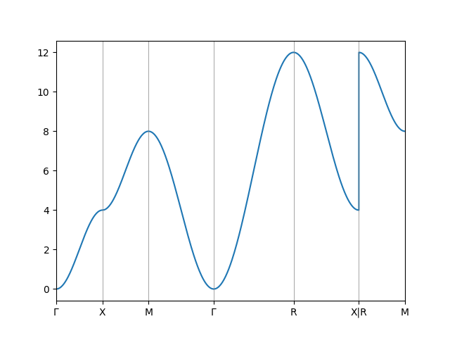
lswt = magnopy.LSWT(spinham, spin_directions=[[0, 0, 1]])
omegas = [lswt.omega(k=kpoint)[0].real for kpoint in kp.points()]

• And for plotting

import matplotlib.pyplot as plt

_, ax = plt.subplots()

ax.plot(kp.flat_points(), omegas)

ax.set_xticks(kp.ticks(), kp.labels)
ax.vlines(kp.ticks(), 0, 1, transform=ax.get_xaxis_transform(), color="grey", lw=0.5)
ax.set_xlim(kp.ticks()[0], kp.ticks()[-1])

plt.show()