(extra) Wulfric

Exercises

• Create a crystal structure, in which conventional and primitive cells are the same. Compute k-points and k-path for it.

• Create a crystal structure, in which original cell is neither conventional nor primitive. Compute k-points and k-path for it.

• For the crystal structure from this page compute k-points and k-path for the (2, 3, 1) super-cell. Compare high-symmetry points and k-path with those of the original cell.

• For the crystal structure from this page compute k-points and k-path for the (2, 3, 1) super-cell, modifying the spglib_types in such a way that same atoms of the original cell that are located in different "sub-cells" of the super-cell have different spglib_types. Compare high-symmetry points and k-path with those of the original cell.

For the upcoming tutorials we need to be able to generate a set of k-points. In particular, a set of k-points for the k-path between high-symmetry points. There is a number of ways to do so and a number of packages out there that can deal with such a task. Magnopy use one of them, wulfric, as a dependency for k-points, symmetry analysis (powered by spglib) and visualization (powered by Plotly).

That is why in the tutorials we will use wulfric for automatic generation of k-points. In this tutorial we briefly introduce it. It is not necessary to use wulfric, please feel free to skip this tutorial if you have other ways to generate k-points.

import numpy as np
import wulfric
import matplotlib.pyplot as plt

# Get a cubic cell with a = 4
cell = 4 * np.eye(3)

# Eight atoms: four will be magnetic, and four will not
atoms = dict(
    names=["Fe1", "Fe2", "Fe3", "Fe4", "O1", "O2", "O3", "O4"],
    positions=[
        [0.0, 0.0, 0.0],
        [0.5, 0.5, 0.0],
        [0.0, 0.5, 0.5],
        [0.5, 0.0, 0.5],
        [0.5, 0.5, 0.5],
        [0.5, 0.0, 0.0],
        [0.0, 0.5, 0.0],
        [0.0, 0.0, 0.5],
    ],
    spins=[2.5, 2.5, 2.5, 2.5, None, None, None, None],
    g_factors=[2, 2, 2, 2, None, None, None, None],
)

Getting symmetry information

Many of wulfric's functions accept optional parameter called spglib_data. Each of them behave in the same way whether such parameter is given or not (if not given, it is created internally). However, if you plan to call multiple wulfric functions that need spglib_data, it is more efficient to create it once and pass it to those functions. You can skip this section if you do not plan to do so.

Hint

Create an spglib_data after you finished modifying the crystal structure. If you modify the crystal structure, then you need to re-create spglib_data.

spglib_data = wulfric.get_spglib_data(cell=cell, atoms=atoms, spglib_symprec=1e-5)

Note

• spglib_symprec is a tolerance parameter for the space group search that is directly passed to spglib, see its docs for more information. Default value 1e-5 is usually good enough. You can try to increase it if your crystal structure is slightly distorted and computed space group is not the one you would expect.

• spglib decides which atoms in the unit cell are equivalent based on spglib_types - a list of positive, non-zero integers. wulfric guesses spglib_types for you, based on the atoms dictionary. See wulfric.get_spglib_types() to read how this guess is done.

Here are the spglib_types, that were guessed by wulfric:

print(spglib_data.original_types)

[1, 1, 1, 1, 2, 2, 2, 2]

If you want to control how spglib_types are defined, then you can add them directly to atoms

atoms["spglib_types"] = [1, 1, 1, 1, 2, 2, 2, 2]

Symmetry information

A number of properties about the underlying crystal can be displayed now

See wulfric.get_spglib_data() for full list of available keys.

print(f"Space group: {spglib_data.space_group_number}")
print(f"Bravais lattice: {spglib_data.crystal_family + spglib_data.centring_type}")

Space group: 225
Bravais lattice: cF

wulfric supports two conventions for the high-symmetry k-points: by Hinuma, Pizzi, Kumagai, Oba, Tanaka (HPKOT) [1] and by Setyawan and Curtarolo (SC) [2]. Magnopy defaults to HPKOT convention internally.

HPKOT convention

hpkot_ebls = wulfric.crystal.hpkot_get_extended_bl_symbol(
    cell=cell, atoms=atoms, spglib_data=spglib_data
)
print(f"Extended Bravais lattice symbol according to HPKOT: {hpkot_ebls}")

hpkot_kpath, hpkot_hs_points = wulfric.kpoints.get_path_and_points(
    cell=cell, atoms=atoms, spglib_data=spglib_data, convention="HPKOT"
)
print(f"Recommended k-path according to HPKOT: {hpkot_kpath}")

# hs_points is a dictionary: {name : coordinate, ...}
print("Pre-defined high symmetry points according to HPKOT:")
for name, rel_pos in hpkot_hs_points.items():
    print(f"* {name:<7} at {rel_pos[0]:>8.5f} {rel_pos[0]:>8.5f} {rel_pos[0]:>8.5f}")

Extended Bravais lattice symbol according to HPKOT: cF2
Recommended k-path according to HPKOT: GAMMA-X-U|K-GAMMA-L-W-X
Pre-defined high symmetry points according to HPKOT:
* GAMMA   at  0.00000  0.00000  0.00000
* X       at  0.00000  0.00000  0.00000
* L       at  0.50000  0.50000  0.50000
* W       at  0.50000  0.50000  0.50000
* W2      at  0.00000  0.00000  0.00000
* K       at  0.75000  0.75000  0.75000
* U       at  0.25000  0.25000  0.25000

SC convention

sc_variation = wulfric.crystal.sc_get_variation(
    cell=cell, atoms=atoms, spglib_data=spglib_data
)
print(f"Bravais lattice variation according to SC: {sc_variation}")

sc_kpath, sc_hs_points = wulfric.kpoints.get_path_and_points(
    cell=cell, atoms=atoms, spglib_data=spglib_data, convention="SC"
)
print(f"Recommended k-path according to  SC: {sc_kpath}")

# hs_points is a dictionary: {name : coordinate, ...}
print("Pre-defined high symmetry points according to SC:")
for name, rel_pos in sc_hs_points.items():
    print(f"* {name:<7} at {rel_pos[0]:>8.5f} {rel_pos[0]:>8.5f} {rel_pos[0]:>8.5f}")

Bravais lattice variation according to SC: FCC
Recommended k-path according to  SC: GAMMA-X-W-K-GAMMA-L-U-W-L-K|U-X
Pre-defined high symmetry points according to SC:
* GAMMA   at  0.00000  0.00000  0.00000
* K       at  0.75000  0.75000  0.75000
* L       at  0.50000  0.50000  0.50000
* U       at  0.25000  0.25000  0.25000
* W       at  0.50000  0.50000  0.50000
* X       at  0.00000  0.00000  0.00000

Coordinates of the high-symmetry points are relative. Read further to find out what are they relative to.

Hint

To get absolute coordinates of the high-symmetry points pass relative=False to wulfric.kpoints.get_path_and_points().

From this point we will use HPKOT convention.

Cell, cell and cell

Please read Which cell? to understand the title of this section.

We typically call spinham.cell "cell" or "unit cell" or "input cell" or "original cell". There is no implication on what kind of cell it can be. In fact, it can be a supercell or a primitive cell or a conventional cell or none of those.

• Conventional cell

  Chosen cell for each space group, that can contain more than one lattice point. Depends on the convention.

• Primitive cell

  Chosen cell for each space group, that contains exactly one lattice point. Depends on the convention.

• Supercell

  A cell that contain several repetitions of the original cell.

Hint

If spglib_types are not modified between cells in the supercell, then any supercell for an arbitrary given cell will have the same primitive and conventional cells.

Here is a visualization (we use wulfric.PlotlyEngine, but exactly the same figure can be done with magnopy.PlotlyEngine).

conv_cell, conv_atoms = wulfric.crystal.get_conventional(
    cell=cell, atoms=atoms, spglib_data=spglib_data, convention="HPKOT"
)

prim_cell, prim_atoms = wulfric.crystal.get_primitive(
    cell=cell, atoms=atoms, spglib_data=spglib_data, convention="HPKOT"
)

pe = wulfric.PlotlyEngine(_sphinx_gallery_fix=True)

pe.plot_cell(cell=cell, legend_label="Original cell", color="#000000")
pe.plot_atoms(
    cell=cell,
    atoms=atoms,
    legend_label="Original atoms",
    colors=["#000000" for _ in atoms["names"]],
)

pe.plot_cell(cell=conv_cell, legend_label="Conventional cell", color="#0057B7")
pe.plot_atoms(
    cell=conv_cell,
    atoms=conv_atoms,
    legend_label="Conventional atoms",
    colors=["#0057B7" for _ in conv_atoms["names"]],
)

pe.plot_cell(cell=prim_cell, legend_label="Primitive cell", color="#FFDD00")
pe.plot_atoms(
    cell=prim_cell,
    atoms=prim_atoms,
    legend_label="Primitive atoms",
    colors=["#FFDD00" for _ in prim_atoms["names"]],
)

pe.show(axes_visible=False, legend_position="left")

Note

• In this example input cell is the conventional cell of the crystal.

• In this example conventional and primitive cells are different.

• Both statements from above are crystal-specific, convention-specific and depend on the choice of the input cell, even for the same crystal and convention.

High-symmetry points and k-path

Now we are ready to answer the question from above: what are relative coordinates of high symmetry points relative to?

Important

• High symmetry k-points returned by wulfric are the high-symmetry points of the Brillouin zone of the primitive cell

• Relative coordinates of high-symmetry points produced by wulfric are given in the basis of (relative to) the reciprocal cell of the input cell

Please take a moment to think about those two statements. They have some subtle consequences, among which are the following

• Wulfric always returns high-symmetry points and k-path appropriate to the symmetry of the given crystal. In other words, they are not defined by just the input cell alone. They can be different for the same cell, if it is paired with different set of atoms (or same set of atoms with different spglib_types).

• High-symmetry points and k-path will be the same for some given cell and all of its super-cells. The relative coordinates of the high-symmetry points will change from supercell to supercell, but absolute ones and names will remain the same.

• If you want to obtain high symmetry points and k-path for any given cell alone, then use it with a "blank" set of atoms, i. e. atoms = dict(spglib_types = [1], positions=[[0, 0, 0]])

We will illustrate those facts below. First, we introduce a convenient interface to the k-points that we will use in the later tutorials: wulfric.Kpoints class.

kp = wulfric.Kpoints.from_crystal(cell=cell, atoms=atoms)

# Coordinates of the high symmetry points ar relative to kp.rcell
print(np.allclose(kp.rcell, wulfric.cell.get_reciprocal(cell=cell)))

True

Note

The simple call to the wulfric.Kpoints.from_crystal() can be improved. For example,

• We could have passed convention="HPKOT" or convention="SC" to wulfric.Kpoints.from_crystal(). "HPKOT" is used by default.

• We could have passed spglib_data=spglib_data to wulfric.Kpoints.from_crystal() to avoid recomputing it internally.

Now we can visualize high-symmetry points and k-path.

kp_of_input_cell = wulfric.Kpoints.from_crystal(
    cell=cell, atoms=dict(spglib_types=[1], positions=[[0, 0, 0]])
)

pe = wulfric.PlotlyEngine(_sphinx_gallery_fix=True)

pe.plot_kpoints(
    kp, color="#C8102E", legend_label="High-symmetry points (crystal-based)"
)
pe.plot_kpath(kp, color="#C8102E", legend_label="Recommended k-path (crystal-based)")
pe.plot_brillouin_zone(
    cell=prim_cell,
    color="#C8102E",
    legend_label="Brillouin zone of the primitive cell",
)


pe.plot_kpoints(
    kp_of_input_cell, color="#003DA5", legend_label="High-symmetry points (cell-based)"
)
pe.plot_kpath(
    kp_of_input_cell, color="#003DA5", legend_label="Recommended k-path (cell-based)"
)
pe.plot_brillouin_zone(
    cell=cell,
    color="#003DA5",
    legend_label="Brillouin zone of the input cell",
)

pe.show(axes_visible=False, legend_position="left")

Using Kpoints class

Finally, after we explained how high-symmetry points and k-path are chosen by wulfric, we give some tips on how to use wulfric.Kpoints both for calculation and for plotting. For illustrative purposes we will create an instance of such class by hand.

Hint

When you are working with an actual crystal structure, we recommend to use wulfric.Kpoints.from_crystal(), for example

kp = wulfric.Kpoints.from_crystal(cell=spinham.cell, atoms=spinham.atoms)

kp = wulfric.Kpoints(
    rcell=np.eye(3),
    coordinates=[[0, 0, 0], [0, 0.5, 0], [0.5, 0.5, 0], [0.5, 0.5, 0.5]],
    names=["GAMMA", "X", "M", "R"],
    labels=[R"$\Gamma$", "X", "M", "R"],
    path="GAMMA-X-M-GAMMA-R-X|M-R",
)

For calculation

wulfric.Kpoints.n controls how many kpoints are inserted between each pair (that connected by "-" in the k-path string) of high symmetry points. It defaults to 100, we change it to 10 for illustrative purposes

kp.n = 10

wulfric.Kpoints.points returns a list of k-points from the k-path with n points inserted in between high-symmetry points. Coordinates are absolute by default

for k_b1, k_b2, k_b3 in kp.points(relative=True):
    print(f"{k_b1:>8.5f} {k_b2:>8.5f} {k_b3:>8.5f}", end="")
    found_close = False
    for name in kp.hs_names:
        if np.allclose(kp.hs_coordinates[name], (k_b1, k_b2, k_b3)):
            found_close = True
            print(f"  <-  {name}")
            break
    if not found_close:
        print()

0.00000  0.00000  0.00000  <-  GAMMA
0.00000  0.04545  0.00000
0.00000  0.09091  0.00000
0.00000  0.13636  0.00000
0.00000  0.18182  0.00000
0.00000  0.22727  0.00000
0.00000  0.27273  0.00000
0.00000  0.31818  0.00000
0.00000  0.36364  0.00000
0.00000  0.40909  0.00000
0.00000  0.45455  0.00000
0.00000  0.50000  0.00000  <-  X
0.00000  0.50000  0.00000  <-  X
0.04545  0.50000  0.00000
0.09091  0.50000  0.00000
0.13636  0.50000  0.00000
0.18182  0.50000  0.00000
0.22727  0.50000  0.00000
0.27273  0.50000  0.00000
0.31818  0.50000  0.00000
0.36364  0.50000  0.00000
0.40909  0.50000  0.00000
0.45455  0.50000  0.00000
0.50000  0.50000  0.00000  <-  M
0.50000  0.50000  0.00000  <-  M
0.45455  0.45455  0.00000
0.40909  0.40909  0.00000
0.36364  0.36364  0.00000
0.31818  0.31818  0.00000
0.27273  0.27273  0.00000
0.22727  0.22727  0.00000
0.18182  0.18182  0.00000
0.13636  0.13636  0.00000
0.09091  0.09091  0.00000
0.04545  0.04545  0.00000
0.00000  0.00000  0.00000  <-  GAMMA
0.00000  0.00000  0.00000  <-  GAMMA
0.04545  0.04545  0.04545
0.09091  0.09091  0.09091
0.13636  0.13636  0.13636
0.18182  0.18182  0.18182
0.22727  0.22727  0.22727
0.27273  0.27273  0.27273
0.31818  0.31818  0.31818
0.36364  0.36364  0.36364
0.40909  0.40909  0.40909
0.45455  0.45455  0.45455
0.50000  0.50000  0.50000  <-  R
0.50000  0.50000  0.50000  <-  R
0.45455  0.50000  0.45455
0.40909  0.50000  0.40909
0.36364  0.50000  0.36364
0.31818  0.50000  0.31818
0.27273  0.50000  0.27273
0.22727  0.50000  0.22727
0.18182  0.50000  0.18182
0.13636  0.50000  0.13636
0.09091  0.50000  0.09091
0.04545  0.50000  0.04545
0.00000  0.50000  0.00000  <-  X
0.50000  0.50000  0.00000  <-  M
0.50000  0.50000  0.04545
0.50000  0.50000  0.09091
0.50000  0.50000  0.13636
0.50000  0.50000  0.18182
0.50000  0.50000  0.22727
0.50000  0.50000  0.27273
0.50000  0.50000  0.31818
0.50000  0.50000  0.36364
0.50000  0.50000  0.40909
0.50000  0.50000  0.45455
0.50000  0.50000  0.50000  <-  R

For plotting

wulfric.Kpoints.flat_points returns a list of flat indices that can be used in the band structure plots. Same length as in wulfric.Kpoints.points.

print(len(kp.points()) == len(kp.flat_points()))

for flat_index, point in zip(kp.flat_points(), kp.points(relative=True)):
    print(f"{flat_index:>8.5f}", end="")

    found_close = False
    for name in kp.hs_names:
        if np.allclose(kp.hs_coordinates[name], point):
            found_close = True
            print(f"  <-  {name}")
            break
    if not found_close:
        print()

True
 0.00000  <-  GAMMA
 0.04545
 0.09091
 0.13636
 0.18182
 0.22727
 0.27273
 0.31818
 0.36364
 0.40909
 0.45455
 0.50000  <-  X
 0.50000  <-  X
 0.54545
 0.59091
 0.63636
 0.68182
 0.72727
 0.77273
 0.81818
 0.86364
 0.90909
 0.95455
 1.00000  <-  M
 1.00000  <-  M
 1.06428
 1.12856
 1.19285
 1.25713
 1.32141
 1.38569
 1.44998
 1.51426
 1.57854
 1.64282
 1.70711  <-  GAMMA
 1.70711  <-  GAMMA
 1.78584
 1.86457
 1.94330
 2.02203
 2.10075
 2.17948
 2.25821
 2.33694
 2.41567
 2.49440
 2.57313  <-  R
 2.57313  <-  R
 2.63741
 2.70170
 2.76598
 2.83026
 2.89454
 2.95883
 3.02311
 3.08739
 3.15167
 3.21596
 3.28024  <-  X
 3.28024  <-  M
 3.32569
 3.37115
 3.41660
 3.46206
 3.50751
 3.55297
 3.59842
 3.64388
 3.68933
 3.73478
 3.78024  <-  R

wulfric.Kpoints.ticks and wulfric.Kpoints.labels return positions and labels of the high-symmetry points. wulfric.Kpoints.ticks are on the same scale as wulfric.Kpoints.flat_points

for tick, label in zip(kp.ticks(), kp.labels):
    print(f"{tick:>8.5f} -> {label}")

0.00000 -> $\Gamma$
0.50000 -> X
1.00000 -> M
1.70711 -> $\Gamma$
2.57313 -> R
3.28024 -> X|M
3.78024 -> R

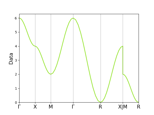
Example

Here is an example of how those attributes can be used.

# Prepare some tricks
a, b, c, _, _, _ = wulfric.cell.get_params(cell=wulfric.cell.get_reciprocal(kp.rcell))

# Use in calculations
points = kp.points()
data = (
    3 + np.cos(a * points[:, 0]) + np.cos(b * points[:, 1]) + np.cos(c * points[:, 2])
)

# Use in plotting
fig, ax = plt.subplots()

ax.plot(kp.flat_points(), data, lw=2, color="#98E534")

ax.set_xticks(kp.ticks(), kp.labels, fontsize=15)
ax.set_ylabel("Data", fontsize=15)

ax.set_xlim(kp.ticks()[0], kp.ticks()[-1])
ax.set_ylim(0, None)

ax.vlines(kp.ticks(), 0, 1, lw=0.5, color="grey", transform=ax.get_xaxis_transform())

fig.show()

References

[1]

Hinuma, Y., Pizzi, G., Kumagai, Y., Oba, F. and Tanaka, I., 2017. Band structure diagram paths based on crystallography. Computational Materials Science, 128, pp.140-184.

[2]

Setyawan, W. and Curtarolo, S., 2010. High-throughput electronic band structure calculations: Challenges and tools. Computational materials science, 49(2), pp. 299-312.