Classical Energy

Exercises

1. Compute classical energy of one of the Hamiltonians from the previous tasks.

2. Change the convention of the spin Hamiltonian and compute the energy again. Does it change?

3. Create a Hamiltonian with the isotropic exchange, triaxial anisotropy and DM interaction. Optimize the spin direction for the full Hamiltonian. Use them to compute energy contributions of every term.

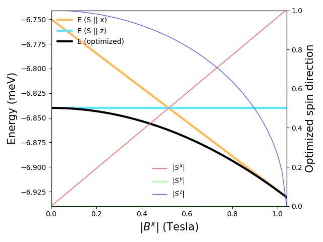
4. (extra) Create a Hamiltonian of the ferromagnet with an easy magnetic axis. Find out numerically the value of the magnetic field that shall be applied perpendicular to the easy axis, which fully orients the spins along the magnetic field.

import numpy as np
import magnopy
import matplotlib.pyplot as plt

Exercise 1

spinham = magnopy.examples.cubic_ferro_nn(S=1, J_iso=1)

print(magnopy.Energy(spinham)([[0, 0, 1]]))

-3.0

Exercise 2

print(spinham.convention)

spinham.convention = spinham.convention.get_modified(c22=0.3333)

print(spinham.convention)

print(magnopy.Energy(spinham)([[0, 0, 1]]))

"custom" convention where
  * Bonds are counted multiple times in the sum;
  * Spin vectors are not normalized;
  * Undefined c1 factor;
  * c21 = 1.0;
  * c22 = 0.5;
  * Undefined c31 factor;
  * Undefined c32 factor;
  * Undefined c33 factor;
  * Undefined c41 factor;
  * Undefined c421 factor;
  * Undefined c422 factor;
  * Undefined c43 factor;
  * Undefined c44 factor.
"custom" convention where
  * Bonds are counted multiple times in the sum;
  * Spin vectors are not normalized;
  * Undefined c1 factor;
  * c21 = 1.0;
  * c22 = 0.3333;
  * Undefined c31 factor;
  * Undefined c32 factor;
  * Undefined c33 factor;
  * Undefined c41 factor;
  * Undefined c421 factor;
  * Undefined c422 factor;
  * Undefined c43 factor;
  * Undefined c44 factor.
-3.0

No, energy, being a physical property, does not depend on Hamiltonians convention.

Exercise 3

# Orthorhombic cell with a = 1, b=1.5, c=2
cell = np.diag([1, 1.5, 2])

# One atom per unit cell
atoms = dict(
    names=["Fe"],
    positions=[[0.0, 0.0, 0.0]],
    spins=[2.5],
    g_factors=[2],
)

# Convention
convention = magnopy.Convention(
    multiple_counting=True, spin_normalized=False, c21=1, c22=1 / 2
)

# Create three terms
iso_term = magnopy.SpinHamiltonian(cell=cell, atoms=atoms, convention=convention)
aniso_term = iso_term.get_empty()
dmi_term = iso_term.get_empty()

# Add nearest neighbor isotropic exchange
for nu in [(1, 0, 0), (0, 1, 0), (0, 0, 1)]:
    iso_term.add_22(
        alpha=0, beta=0, nu=nu, parameter=magnopy.converter22.from_iso(iso=-1)
    )

# Add triaxial anisotropy
aniso_term.add_21(alpha=0, parameter=np.diag([-0.1, -0.3, -0.2]))

# Add DMI to one of the nearest neighbors
dmi_term.add_22(
    alpha=0,
    beta=0,
    nu=(0, 1, 0),
    parameter=magnopy.converter22.from_dmi(dmi=(0.5, 0, 0)),
)

# Get an energy instance for the full Hamiltonian
energy_full = magnopy.Energy(iso_term + aniso_term + dmi_term)

# Get optimized spin directions
optimized_sd = energy_full.optimize()

print(f"Optimized spin directions are\n{optimized_sd}")

# Print energy contributions
print(f"Total energy is {energy_full(optimized_sd):.4f} meV")
print(f"Isotropic contribution is {magnopy.Energy(iso_term)(optimized_sd):.4f} meV")
print(f"Anisotropic contribution is {magnopy.Energy(aniso_term)(optimized_sd):.4f} meV")
print(f"DMI contribution is {magnopy.Energy(dmi_term)(optimized_sd):.4f} meV")

─────┬─────────────┬─────────────┬─────────────
step │     E_0     │  delta E_0  │ max torque
─────┴─────────────┴─────────────┴─────────────
1      -20.6106991     0.1218815     0.1976675
2      -20.6236014     0.0129023     0.0665848
3      -20.6249387     0.0013373     0.0160851
4      -20.6250000     0.0000613     0.0003449
5      -20.6250000     0.0000000     0.0000089
───────────────────────────────────────────────
Optimized spin directions are
[[-2.50504806e-06 -1.00000000e+00 -5.10432729e-06]]
Total energy is -20.6250 meV
Isotropic contribution is -18.7500 meV
Anisotropic contribution is -1.8750 meV
DMI contribution is 0.0000 meV

Exercise 4

Hint

Magnetic field tends to orient magnetic moment along itself, but the spin along the opposite direction.

# Create a Hamiltonian
# Parameters are in meV by default
spinham = magnopy.examples.cubic_ferro_nn(S=3 / 2, J_iso=1, J_21=np.diag([0, 0, -0.04]))

# Create a Zeeman term with the small magnetic field step value of (-0.02, 0, 0) Tesla
zeeman_step = spinham.get_empty()
print(f"Number of atoms: {len(zeeman_step.atoms.names)} -> {zeeman_step.atoms.names}")
B_step = -0.02
zeeman_step.add_magnetic_field(B=(B_step, 0, 0), alphas=[0])

energy = magnopy.Energy(spinham)

# Lists for saving the intermediate steps
energies_along_z = [energy([[0, 0, 1]])]
energies_along_x = [energy([[1, 0, 0]])]
optimized_sds = [energy.optimize(quiet=True)]
energies_optimized = [energy(optimized_sds[-1])]

steps = 0
# Avoid using S^x == 1, due to the numerical noise
while abs(optimized_sds[-1][0][0]) < 0.9999:
    # Increase magnetic field
    spinham = spinham + zeeman_step
    steps += 1

    # Update energy
    energy = magnopy.Energy(spinham)

    # Save info about the step
    energies_along_z.append(energy([[0, 0, 1]]))
    energies_along_x.append(energy([[1, 0, 0]]))
    optimized_sds.append(energy.optimize(quiet=True))
    energies_optimized.append(energy(optimized_sds[-1]))

print(f"({B_step * steps:.4f}, 0.0, 0.0) Tesla is enough.")

Number of atoms: 1 -> ['X']
(-1.0400, 0.0, 0.0) Tesla is enough.

Plot the results as well

Hint

We display absolute values of spin components as +z and -z are degenerate in the model and optimized directions will oscillate is raw value is plotted.

B_x = np.abs([_ * B_step for _ in range(steps + 1)])
optimized_sds = np.array(optimized_sds)

fig, ax = plt.subplots()

# Plot energies
ax.plot(B_x, energies_along_x, label="E (S || x)", lw=3, color="#FFB956")
ax.plot(B_x, energies_along_z, label="E (S || z)", lw=3, color="#53EBFF")
ax.plot(B_x, energies_optimized, label="E (optimized)", lw=3, color="#000000")

ax.set_xlabel(R"$|B^x|$ (Tesla)", fontsize=15)
ax.set_ylabel(R"Energy (meV)", fontsize=15)
ax.set_xlim(B_x[0], B_x[-1])

ax.legend(frameon=False, loc="upper left")

# Plot optimized spin directions
twinax = ax.twinx()

twinax.plot(
    B_x, np.abs(optimized_sds[:, 0, 0]), label=R"$|S^x|$", lw=1, color="#FF5656"
)
twinax.plot(
    B_x, np.abs(optimized_sds[:, 0, 1]), label=R"$|S^y|$", lw=1, color="#67FF56"
)
twinax.plot(
    B_x, np.abs(optimized_sds[:, 0, 2]), label=R"$|S^z|$", lw=1, color="#5659FF"
)

twinax.set_ylabel(R"Optimized spin direction", fontsize=15)
twinax.set_ylim(0, 1)

twinax.legend(frameon=False, loc="lower center")

fig.tight_layout()
fig.show()