Linear Spin Wave theory

Exercises

1. Compute magnon dispersion of a simple ferromagnet.

2. Compute magnon dispersion of a simple antiferromagnet.

import numpy as np
import magnopy
import wulfric
import matplotlib.pyplot as plt

Exercise 1

# Cubic cell with a = 1
cell = np.eye(3)

# One atom per unit cell in the center of the cell
atoms = dict(
    names=["Fe"],
    positions=[[0.5, 0.5, 0.5]],
    spins=[1.0],
    g_factors=[2.0],
)

# Choose a convention
convention = magnopy.Convention(
    multiple_counting=True, spin_normalized=False, c21=1, c22=1
)

# Create an empty spin Hamiltonian
spinham = magnopy.SpinHamiltonian(cell=cell, atoms=atoms, convention=convention)

# Add a Heisenberg exchange interaction between nearest neighbors
parameter = magnopy.converter22.from_iso(iso=-1.0)  # Ferromagnetic exchange

for nu in [(1, 0, 0), (0, 1, 0), (0, 0, 1)]:
    spinham.add_22(alpha=0, beta=0, nu=nu, parameter=parameter)

# Add an on-site anisotropy term
spinham.add_21(alpha=0, parameter=np.diag([0.0, 0.0, -0.5]))

# Visualize the spin Hamiltonian
pe1, pe2 = magnopy.experimental.plot_spinham(spinham=spinham, _sphinx_gallery_fix=True)

On-site terms

pe1.show(axes_visible=False)

Bilinear terms

pe2.show(axes_visible=False)

Next, work with linear spin wave theory to compute magnon dispersion.

# Create a linear spin wave theory object
lswt = magnopy.LSWT(spinham=spinham, spin_directions=[[0, 0, 1]])

# Get high-symmetry points
kp = wulfric.Kpoints.from_crystal(cell=spinham.cell, atoms=spinham.atoms)
kp.n = 20

omegas = np.array(
    [lswt.omega(k=k, relative=False) for k in kp.points(relative=False)]
).T.real

# Plot the magnon dispersion

fig, ax = plt.subplots()

for omega in omegas:
    ax.plot(kp.flat_points(), omega)

ax.set_xlim(kp.ticks()[0], kp.ticks()[-1])
ax.set_ylim(0, None)

ax.set_xticks(kp.ticks(), kp.labels, fontsize=15)
ax.vlines(
    kp.ticks(),
    0,
    1,
    color="grey",
    lw=0.5,
    transform=ax.get_xaxis_transform(),
)

ax.set_ylabel("Energy (meV)", fontsize=15)
ax.set_title("Magnon Dispersion - Simple Ferromagnet", fontsize=15)

fig.tight_layout()
fig.show()

Exercise 2

For this exercise, we will make a model for the 1D chain antiferromagnet with an easy magnetic axis along \(\mathbf{z}\).

# Cubic cell with a = 2
cell = np.eye(3)

# Two atoms per unit cell
atoms = dict(
    names=["Fe1", "Fe2"],
    positions=[[0.25, 0.5, 0.5], [0.75, 0.5, 0.5]],
    spins=[1.0, 1.0],
    g_factors=[2.0, 2.0],
    # Different, to get correct high-symmetry points and k-path
    spglib_types=[1, 2],
)

# Choose a convention
convention = magnopy.Convention(
    multiple_counting=True, spin_normalized=False, c21=1, c22=1
)

# Create an empty spin Hamiltonian
spinham = magnopy.SpinHamiltonian(cell=cell, atoms=atoms, convention=convention)

# Add a Heisenberg exchange interaction between nearest neighbors
parameter = magnopy.converter22.from_iso(iso=1.0)  # Antiferromagnetic exchange

# No need to add all four bonds, the rest are generated automatically
spinham.add_22(alpha=0, beta=1, nu=(0, 0, 0), parameter=parameter)
spinham.add_22(alpha=0, beta=1, nu=(-1, 0, 0), parameter=parameter)

# Add an on-site anisotropy term, to both atoms
spinham.add_21(alpha=0, parameter=np.diag([0.0, 0.0, -0.1]))
spinham.add_21(alpha=1, parameter=np.diag([0.0, 0.0, -0.1]))

# Add some magnetic field to lift the degeneracy of the modes
spinham.add_magnetic_field(B=(0, 0, 1))


# Visualize the spin Hamiltonian
pe1, pe2 = magnopy.experimental.plot_spinham(spinham=spinham, _sphinx_gallery_fix=True)

On-site terms

pe1.show(axes_visible=False)

Bilinear terms

pe2.show(axes_visible=False)

Next, work with linear spin wave theory to compute magnon dispersion.

# Create a linear spin wave theory object
lswt = magnopy.LSWT(spinham=spinham, spin_directions=[[0, 0, 1], [0, 0, -1]])

# Get high-symmetry points
kp = wulfric.Kpoints.from_crystal(cell=spinham.cell, atoms=spinham.atoms)
kp.n = 20

for name, pos in zip(kp.hs_names, kp.hs_coordinates.values()):
    print(f"{name}: {pos}")

omegas = np.array(
    [lswt.omega(k=k, relative=False) for k in kp.points(relative=False)]
).T.real

# Plot the magnon dispersion

fig, ax = plt.subplots()

for omega in omegas:
    ax.plot(kp.flat_points(), omega)

ax.set_xlim(kp.ticks()[0], kp.ticks()[-1])
ax.set_ylim(0, None)

ax.set_xticks(kp.ticks(), kp.labels, fontsize=15)
ax.vlines(
    kp.ticks(),
    0,
    1,
    color="grey",
    lw=0.5,
    transform=ax.get_xaxis_transform(),
)

ax.set_ylabel("Energy (meV)", fontsize=15)
ax.set_title("Magnon Dispersion - Simple Antiferromagnet", fontsize=15)

fig.tight_layout()
fig.show()

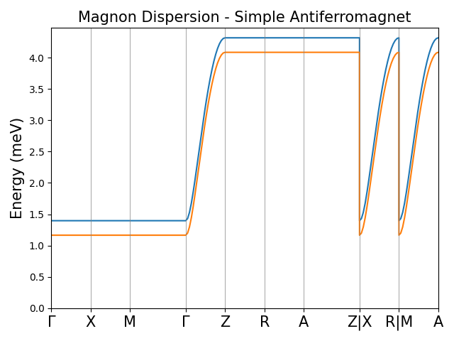
GAMMA: [0. 0. 0.]
Z: [0.5 0.  0. ]
M: [0.  0.5 0.5]
A: [0.5 0.5 0.5]
R: [0.5 0.  0.5]
X: [0.  0.  0.5]