Getting files for Vampire

This tutorial is a special one. It does not require you to finish any task and give all the code that you need to execute. You can copy a notebook for this tutorial from the Tutorial_2/magnopy-vampire-link folder.

In order to run a simulation with Vampire, using parameters of a material, that were computed by GROGU or TB2J one have to convert the data from those codes to the material file (.mat) and unit cell file (.UCF) of Vampire.

Reference files can be downloaded here

• For for "CrI3/reference-GROGU.txt"

  • CrI3/reference-GROGU.txt

  • Vampire_CrI3.mat (for CrI3.txt)

  • Vampire_CrI3.UCF (for CrI3.txt)

• For for "CrI3_U/reference-GROGU.txt"

  • CrI3_U/reference-GROGU.txt

  • Vampire_CrI3_U.mat (for CrI3_U.txt)

  • Vampire_CrI3_U.UCF (for CrI3_U.txt)

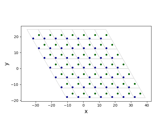
There is one complication that arises with it. By design Vampire accepts only rectangular unit cells and CrI3 unit cell is not a rectangular one. Here is a visualization of it

import magnopy
import matplotlib.pyplot as plt
import numpy as np

# Change those variables to convert other files
INPUT_FILE = "../../resources/trilmax-2025/CrI3/reference-GROGU.txt"
VAMPIRE_SEEDNAME = "Vampire_CrI3"

# INPUT_FILE = "../../resources/trilmax-2025/CrI3_U/reference-CrI3.txt"
# VAMPIRE_SEEDNAME = "Vampire_CrI3_U"

spinham = magnopy.io.load_grogu(INPUT_FILE)
pe = magnopy.PlotlyEngine(_sphinx_gallery_fix=True)
pe.plot_cell(cell=spinham.cell)
pe.plot_atoms(cell=spinham.cell, atoms=spinham.atoms)
pe.show(height=500)

Let us plot it in 2D, for simplicity

# Put first atom exactly in the corner
spinham.atoms.positions = (
    spinham.atoms.positions - np.array(spinham.atoms.positions)[0][np.newaxis, :]
)
# Shift all atoms in the middle of the unit cell along a3
spinham.atoms.positions[:, 2] = spinham.atoms.positions[:, 2] + 0.5

# Shift all atoms a little bit along a1 and a2
spinham.atoms.positions[:, 0] = spinham.atoms.positions[:, 0] + 0.1
spinham.atoms.positions[:, 1] = spinham.atoms.positions[:, 1] + 0.1


def plot_cell(ax, a1, a2, shift=(0, 0, 0)):
    shift = np.array(shift)
    A = shift
    B = shift + a1
    C = shift + a1 + a2
    D = shift + a2

    box = np.array([A, B, C, D, A]).T

    ax.plot(
        box[0],
        box[1],
        lw=1,
        color="lightgrey",
        zorder=1,
    )


abs_positions = spinham.atoms.positions @ spinham.cell
a1, a2, a3 = spinham.cell

fig, ax = plt.subplots()
for i in range(-3, 4):
    for j in range(-3, 4):
        shift = a1 * i + a2 * j
        ax.plot(
            abs_positions[0][0] + shift[0],
            abs_positions[0][1] + shift[1],
            "o",
            color="darkblue",
            ms=4,
            zorder=2,
        )
        ax.plot(
            abs_positions[1][0] + shift[0],
            abs_positions[1][1] + shift[1],
            "o",
            color="darkgreen",
            ms=4,
            zorder=2,
        )
        plot_cell(ax=ax, shift=shift, a1=a1, a2=a2)
ax.set_aspect(1)
ax.set_xlabel("x", fontsize=15)
ax.set_ylabel("y", fontsize=15)
fig.show()

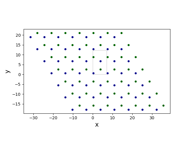
Now, choose the rectangular cell by connecting four atoms:

• (0, (0, 0, 0))

• (0, (1, 0, 0))

• (0, (2, 2, 0))

• (0, (1, 2, 0))

where the syntax is (atom_index, (i, j, k)). Then, new unit cell can be chosen as

new_a1 = a1
new_a2 = a1 + 2 * a2

fig, ax = plt.subplots()
plot_cell(ax, a1=new_a1, a2=new_a2)

for i in range(-3, 4):
    for j in range(-3, 4):
        shift = a1 * i + a2 * j
        ax.plot(
            abs_positions[0][0] + shift[0],
            abs_positions[0][1] + shift[1],
            "o",
            color="darkblue",
            ms=4,
            zorder=2,
        )
        ax.plot(
            abs_positions[1][0] + shift[0],
            abs_positions[1][1] + shift[1],
            "o",
            color="darkgreen",
            ms=4,
            zorder=2,
        )
ax.set_aspect(1)
ax.set_xlabel("x", fontsize=15)
ax.set_ylabel("y", fontsize=15)
fig.show()

New set of four atoms, that is associated with the new cell can be described as

• (0, (0, 0, 0))

• (1, (0, 0, 0))

• (0, (1, 1, 0))

• (1, (0, 1, 0))

Use magnopy's experimental feature to change the unit cell of the spin Hamiltonian

new_spinham = magnopy.experimental.change_cell(
    spinham=spinham,
    new_cell=[new_a1, new_a2, a3],
    new_atoms_specs=[(0, (0, 0, 0)), (1, (0, 0, 0)), (0, (1, 1, 0)), (1, (0, 1, 0))],
)

print(len(spinham.p22), len(new_spinham.p22))

assert 2 * len(spinham.p22) == len(new_spinham.p22)

72 144

Finally, use magnopy's io module to save Vampire's files

magnopy.io.dump_vampire(
    spinham=new_spinham, seedname=VAMPIRE_SEEDNAME, materials=[0, 0, 0, 0]
)

Bonus

You can use another experimental feature of magnopy to visualize two Hamiltonians and check that new cell is rectangular and the interactions are reasonable

pe1, pe2 = magnopy.experimental.plot_spinham(
    spinham=spinham, distance_digits=2, _sphinx_gallery_fix=True
)
pe1_new, pe2_new = magnopy.experimental.plot_spinham(
    spinham=new_spinham, distance_digits=2, _sphinx_gallery_fix=True
)

On-site terms. Original Hamiltonian

pe1.show(axes_visible=False)

And new Hamiltonian

pe1_new.show(axes_visible=False)

Exchange terms. Original Hamiltonian

pe2.show(axes_visible=False, legend_position="left")

And new Hamiltonian

pe2_new.show(axes_visible=False, legend_position="left")